Chapter 4 Expectations
4.1 Expectation of a RV
The sample mean is a useful measure of centrality of a set of data and we would like a similar quantity for a distribution.
Suppose we have a sample from a distribution that can take on integer values in the range of \(1\) to \(5\). For example suppose we have the data \(\{ 1,1,2,3,3,3,4,5 \}\). Then the sample mean is \[\begin{aligned} \bar{x} &= \frac{1}{n} \sum_{j=1}^n x_j = \frac{1}{8} (1+1+2+3+3+3+4+5)\\ &= \sum_{i=1}^5 \hat{p}_i \;i = \left(\frac{2}{8} \cdot 1 \right) + \left(\frac{1}{8} \cdot 2 \right) + \left(\frac{3}{8} \cdot 3 \right) + \left(\frac{1}{8} \cdot 4 \right) + \left(\frac{1}{8} \cdot 5 \right) \end{aligned}\] where \(\hat{p}_i\) values are the observed proportions for each possible value. If we have a really large sample then \(\hat{p}_i \approx Pr(X=i)\) and it is natural to define the Expected Value as \[E(X) = \begin{cases} \sum x \, f(x) \;\;\;\;\;\;\;\;\;\;\;\; \textrm{ if } X \textrm{ is discrete} \\ \int_{-\infty}^\infty x \, f(x) \,dx \;\;\;\;\; \textrm{ if } X \textrm{ is continuous} \end{cases}\]
We need to be careful to avoid the \(\infty - \infty\) case and note that if \[\sum_{\textrm{Negative }x} x\,f(x) = -\infty \;\;\;\;\; \textrm{ and } \;\;\;\;\;\sum_{\textrm{Positive }x} x\,f(x) = \infty\] or \[\int_{-\infty}^0 x\,f(x)\, dx = -\infty \;\;\;\;\;\; \textrm{ and } \;\;\;\;\;\int_{0}^\infty x\,f(x)\,dx = \infty\] then the resulting expectation could be written as \(-\infty + \infty\) and that quantity does not exist.
Example Suppose that the lifetime, \(X\), of an appliance has a pdf \[f(x) = 2 e^{-2x}\;\cdot I(x>0)\] Then the expectation of \(X\) is \[E(X) = \int_{-\infty}^{\infty} x \,f(x) \, dx = \int_0^\infty x \, 2e^{-2x} \, dx = 2\int_0^\infty x \, e^{-2x} \, dx\] To finish solving this integral, we need to do integration by parts letting \[\begin{aligned} u =2x & \;\;\;\;& dv = e^{-2x}\,dx \\ du= 2\,dx & & v = -\frac{1}{2} e^{-2x} \end{aligned}\] and therefore \[\begin{aligned} E(X) &= -xe^{-2x} \Big\vert_0^\infty+ \int_0^\infty e^{-2x}\,dx \\ &= 0 + -\frac{1}{2} e^{-2x} \Big\vert_0^\infty \\ &= \frac{1}{2} \end{aligned}\]
Expectations of functions of a RV Suppose we have a random variable \(X\) and some function \(Y=r(X)\), then I might want to know the expectation of the random variable \(Y\). We could just derive the pdf of \(Y\) and calculate its expectation, but that is just a bunch of integration and differentiation that cancels out because (in the continuous case and assuming \(r(x)\) is invertable) \[\begin{aligned} E(Y) &= \int y \, g(y) \, dy \\ &= \int r(x)\, f\big( r(x) \big) \Bigg\vert \frac{dx}{dy} \Bigg\vert \,dy \\ &= \int r(x)\, f(x) \,dx \end{aligned}\]
We could prove that if the expectation of \(Y=r(X)\) exists, then for any function \(r(x)\) is equal to \[E(Y) = E[r(X)] = \begin{cases} \sum r(x) \,f(x) \\ \int r(x) \,f(x) \, dx \end{cases}\]
Example Suppose that we have a random variable with pdf \[f(x) = 3x^2 \, I(0<x<1)\] then \[E(X) = \int_0^1 x\, f(x) \,dx = \int_0^1 x \, 3x^2 \,dx = \int_0^1 3 x^3 \, dx = \frac{3}{4}x^4 \Bigg\vert_0^1 = \frac{3}{4}\] and if we consider \(Y=X^2\) then \[E(Y) = E(X^2) = \int_0^1 x^2\, f(x)\, dx = \int_0^1 3x^4 = \frac{3}{5}x^5\Bigg\vert_0^1 = \frac{3}{5}\]
Notice that \(E(X^2) \ne \Bigg( E(X) \Bigg)^2\). For general \(r(X)\), we typically see that \(E(r(X)) \ne r\Bigg( E(X) \Bigg)\). However for linear functions, it is true.
Suppose that \(X\) has a Uniform(\(a\), \(b\)) distribution. Find the expected value of \(X\).
Suppose that \(X\) has a Uniform(\(a\), \(b\)) distribution. Find the expected value of \(Y=\sqrt X\).
Suppose that \(X\) has a Uniform(\(a\), \(b\)) distribution. Find the expected value of \(Y=1/X\).
A 1-meter stick is broken at a random spot along the stick. Find the expected value of the length of the longer piece.
Expectations of functions of several variables Suppose that a multivariate distribution with joint pdf \(f(x_1, x_2, \dots, x_n)\) and we define \(Y=r(X_1,X_2,\dots,X_n)\) then \[E(Y) = \iint\dots\int r(x_1, x_2, \dots, x_n)\, f(x_1, x_2, \dots, x_n)\, dx_1 dx_2 \dots dx_n\] Example Suppose that we have a bivariate distribution \[f(x_1, x_2) = 8x_1 x_2 \, \cdot I(0 < x_1 < x_2 < 1)\] and we wish to know the expectation of \(Y=X_1+X_2\). Then \[\begin{aligned} E( X_1+X_2 ) &= \int_0^1 \int_0^{x_2} (x_1+x_2) \, 8x_1x_x \; dx_1 dx_2 \\ &= \vdots \\ &= \frac{4}{3} \end{aligned}\]
4.2 Properties of Expectations
Prove that for finite constants \(a\) and \(b\) and continuous random variable \(X\), we have \[E(aX + b) = aE(X) + b\]
Show that if continuous random variable \(X\) has support on the interval \((a,b)\) where \(a<b\), then \(a < E(X) < b\). This is true in the discrete case as well.
Show that if \(X_1\) and \(X_2\) are (possibly not independent!) continuous random variables with joint pdf \(f(x_1, x_2)\) that \(E( X_1 + X_2 ) = E(X_1) + E(X_2)\). By induction this result will hold for the sum of a finite number number random variables. Notice the proof for the discrete case is similar with simply replacing integrals with summations.
Suppose that three random variables \(X_1, X_2, X_3\) are sampled from a distribution that has mean \(E(X_i)=5\). Find the expectation of \(2X_1 - 3X_2 -X_3 - 5\). When we say \(X_1, X_2, \dots\) are sampled from a distribution, we actually mean that \(X_1,X_2,\dots\) are independent and each have marginal distribution as given. So when you heard “We sampled from population …” in your Introduction to Statistics course, they actually were telling you that the observations are independent.
Suppose that three random variables \(X_1, X_2, X_3\) are sampled from a uniform distribution on \((0,1)\). What is the expectation of \((X_1 - 2X_2 + X_3)^2\).
Bernoulli Expectation Suppose that the random variable \(X_i\) can take on values \(0\) or \(1\) and the probability it takes on \(1\) is \(f(1)=p\). What is the expected value of \(X_i\)?
Binomial Expectation Suppose that we have \(n\) identically distributed Bernoulli random variables, each of which having probability of success \(f_i(1)=p\). Letting \(Y=\sum_1^n X_i\), what is the expected value of \(Y\)?
- Hypergeometric Expectation Suppose that we have a bag with \(N\) balls, of which \(M\) are red and \(N-M\) are blue. We will draw \(n\) balls out (without replacement) and we are interested in the total number of red balls drawn. Let \(X_i\) be \(1\) if the \(i\)th draw was a red ball.
- First consider the case where we draw \(n=1\) ball. What is the probability that we draw a red ball on the first draw and therefore what is \(E(X_1)\)?
- Next consider the case where we draw \(n=2\) balls. What is the probability that we draw a red ball on the second draw and therefore what is \(E(X_2)\)?
- The same pattern holds for the rest of \(X_3, X_4, \dots X_n\). Given that, what is the expected value of \(Y=\sum_1^n X_i\)?
Suppose that continuous random variables \(X_1, X_2, \dots, X_n\) are independent, each having a marginal pdf \(f_i(x_i)\). Show that \[E\left( \prod_{i=1}^n X_i \right) = \prod_{i=1}^n E(X_i)\] Notice that this result requires that the variables are independent, whereas the result in 4.2.3 did not require independence.
A gambler will play a game where he is equally likely to win or lose on a given play. When the gambler wins, her fortune is doubled, but when she loses, it is cut in half. Given that the gambler started the game with a fortune of \(c\), what is the expected fortune after \(n\) plays?
It can be shown that for non-negative, continuous random variables \[E(X) = \int_0^\infty (1-F(x))\,dx\] and for non-negative discrete random variables \[E(X) = \sum_{x=1}^\infty Pr( X \ge x )\]
The proof in the discrete case is a reordering of \[E(X) = \sum_{x=0}^\infty x\,f(x) = \sum_x^\infty x\, Pr(X=x)\] to summing one copy of \(Pr(X=1)\) and two copies of \(Pr(X=2)\) and three copies of \(Pr(X=3)\) and so on.
| \(E(X)\) | = | 0 | \(+ Pr(X=1)\) | \(+Pr(X=2)\) | \(+Pr(X=3)\) | \(\dots\) |
| \(+Pr(X=2)\) | \(+Pr(X=3)\) | \(\dots\) | ||||
| \(+Pr(X=3)\) | \(\dots\) | |||||
| \(\ddots\) |
Notice that the first row of this sum is \(Pr(X\ge1)\) and the second is \(Pr(X\ge 2)\) and that establishes the result.
Geometric Expectation Suppose that each time a person plays a game, they have a probability \(p\) of winning. Let the random variable \(X\) be the number of games played until the person wins. We have previously shown that \[f(x) = (1-p)^{x-1}p \;\; I(x\in \{1,2,\dots\})\] \[Pr(X \le x) = 1 - (1-p)^x\] for \(x \in \{1,2,\dots\}\) What is expected number of times a player must play until they win?
Gamma Expectation Suppose that we have a random variable \(X\) with a \(Gamma(\alpha, \beta)\) distribution and therefore \[f(x) = \frac{\beta^\alpha}{\Gamma(\alpha)} x^{\alpha-1} e^{-x\beta} \;\cdot I(x>0)\] Show that \[E(X) = \frac{\alpha}{\beta}\]
4.3 Variance
Although the mean of a distribution is quite useful, it is not the only measure of interest. A secondary measure of interest is a measure of spread of the distribution. Just as the sample variance is interpreted as the “typical squared distance to the mean” we will define the distribution variance as the “expected squared distance to the mean”.
For notational convenience, let \(\mu=E(X)\) and define \[Var(X) = E\big[ (X-\mu)^2 \big]\]
Because expectations don’t necessarily exist, we’ll say that \(Var(X)\) does not exist if \(E(X)\) does not exist or if \(E[(X-\mu)^2]\) does not exist. Notice that the Variance is non-negative because of the square.
Finally, we will define the standard deviation of \(X\) as the positive square-root of the variance. That is \(StdDev(X) = \bigg\vert \sqrt{Var(X)} \bigg\vert\).
Notationally all of this is a bit cumbersome and we’ll use \[E(X) = \mu_X\;\;\;\;\;\;\;\;\;\; Var(X) = \sigma^2_X \;\;\;\;\;\;\;\;\;\; StdDev(X) = \sigma_X\] If we have only a single random variable in a situation, we will suppress the subscript.
- Suppose that RV \(X\) has \(Var(X)\) that exists, then for constants \(a\) and \(b\), show that the RV \[Y=aX+b\] has variance \[Var(Y) = a^2 Var(X)\] Notice that shifting the entire distribution of \(X\) by some constant \(b\) does not affect the spread of the shifted distribution.
Next we consider the sum of independent random variables \(X_1+X_2\). \[\begin{aligned} Var( X_1 + X_2 ) &= E\Bigg[ \bigg[ (X_1 + X_2) - E(X_1+X_2) \bigg]^2 \Bigg] \\ &= E\Bigg[ \bigg[ X_1 + X_2 - \mu_1 - \mu_2 \bigg]^2 \Bigg] \\ &= E\Bigg[ \bigg[ (X_1 -\mu_1) + (X_2 - \mu_2)\bigg]^2 \Bigg] \\ &= E\Bigg[ (X_1 -\mu_1)^2 + 2(X_1-\mu_1)(X_2-\mu_2) + (X_2 - \mu_2)^2 \Bigg] \\ &= E\big[ (X_1 -\mu_1)^2 \big] + E\big[ 2(X_1-\mu_1)(X_2-\mu_2)\big] + E\big[(X_2 - \mu_2)^2 \big] \\ &= Var(X_1) \;\;\;\;\;\;\;\;\;+ 2E\big[ (X_1-\mu_1)(X_2-\mu_2)\big] + Var(X_2) \end{aligned}\] Because \(X_1\) and \(X_2\) are independent then \[E\big[ (X_1-\mu_1)(X_2-\mu_2)\big] = E[(X_1-\mu_1)] E[(X_2-\mu_2)] = (\mu_1 -\mu_1) (\mu_2-\mu_2) = 0\] Repeating this argument for \(n\) independent random variables, we therefore have \[Var( X_1+X_2+\dots+X_n ) = Var(X_1) + Var(X_2) + \dots + Var(X_n)\] \[Var\Bigg( \sum_{i=1}^n X_i \Bigg) = \sum_{i=1}^n Var(X_i)\] Notice that this result requires independence so that the cross-product terms are zero!
Show that \(Var(X) = E(X^2) - \mu^2\). This formula is far more convenient to use, generally.
Suppose that \(X\) has a uniform distribution on the interval \([0,1]\). Compute the variance of \(X\).
Suppose that \(Y\) has a uniform distribution on the interval \([a,b]\) where \(a<b\). Compute the variance of \(Y\).
Suppose that \(X\) has expectation \(\mu\) and variance \(\sigma^2\). Show that \[E\bigg[ X(X-1) \bigg]=\mu(\mu-1) + \sigma^2\]
Suppose that \(X\) has a \(Gamma(\alpha,\beta)\) distribution. Find that the variance of \(X\) is \(\frac{\alpha}{\beta^2}\).
Suppose that \(X\) has a \(Bernoulli(p)\) distribution, that is \(X\) takes on values \(1\) or \(0\) with probabilities \(Pr(X=1)=p\) and \(Pr(X=0) = 1-p\). Find the variance of \(X\).
Suppose that \(Y\) has a \(Binomial(n,p)\) distribution. That is that \[Y=\sum_{i=1}^n X_i\] where \(X_i\) are independent \(Bernoulli(p)\) random variables. Show that \[Var(Y) = np(1-p)\]
4.4 Moments and Moment Generating Functions
Definition 4.1 Just as the \(E(X)\) defines the center of a distribution and \(E[ (X-\mu)^2 ] = E(X^2)-\mu^2\) defines the variance, the quantities \[M_k = E\big( X^k \big)\;\;\;\;\;\;\textrm{ where } k\in \{1,2,3,\dots\}\]
are what we call the \(k\)th moment of the distribution. These moments define other attributes of the distribution, but sometimes it is useful to define a similar quantity called the \(k\)th central moment \[m_k = E\big( ( X-\mu ) ^k \big)\;\;\;\;\;\;\textrm{ where } k\in \{1,2,3,\dots\}\]These two quantities can define several aspects of the distribution. For example, \(M_1=E(X)\) is the distribution mean, while \(M_2=E(X^2)\) is related to the variance. Other attributes are related to higher moments (e.g. the distribution skew is related to \(m_3\)).
Somewhat obnoxiously, the book defines \(M_k\) to exist if and only if \(E\Big(|X|^k\Big) < \infty\). (This is obnoxious because we used a different criteria to say if \(E(X)\) existed in section 4.1 and the definition for the \(k\)th moment is a more strict requirement.)
Suppose that the random variable \(X\) has an \(Exponential(\beta)\) distribution which is a special case of the Gamma distribution. \(Exponential(\beta) = Gamma(1,\beta)\) distribution. The table of distributions in your book shows that the \(Var(X)=\frac{1}{\beta^2}\). Derive the mgf of the Exponential distribution and use it to derive both the expectation and variance.
Mgf of a linear transformation Suppose that we have a random variable \(X\) with mgf \(\psi_1(t)\). Show that \(Y=aX+b\) for real constants \(a\) and \(b\) has the mgf \[\psi_2(t) = e^{bt}\psi_1(at)\]
Suppose that \(X \sim Exponential(\beta)\). Show that \(Y=2X\) has the mgf of an \(Exponential(\beta/2)\) distribution and therefore \(Y \sim Exponential(\beta/2)\).
Derive the moment generating function of the \(Gamma(\alpha, \beta)\) distribution.
Derive the moment generating function of \(Bernoulli(p)\) distribution.
Suppose that independent random variables \(X_1, X_2, \dots, X_n\) each have mgfs \(\psi_1(t), \psi_2(t), \dots, \psi_n(t)\). Show that the mgf of \(Y=\sum X_i\) is \[\psi_Y(t) = \prod_{i=1}^n \psi_i(t)\]
Suppose that \(X_1, X_2, \dots, X_n\) are independent \(Bernoulli(p)\) random variables. Derive the mgf of \(Y=\sum X_i\). That is, derive the mgf of the Binomial distribution.
Suppose that random variable \(X\) has support on the non-negative integers \(0, 1, 2, \dots\). The probability function of \(X\) is \[f(x)=\frac{\lambda^x}{x!}e^{-\lambda}\,\cdot I(x\in \{0,1,2,\dots\})\] The random variable \(X\) has a \(Poisson(\lambda)\) distribution. Derive the mgf of this distribution. Hint: what is the summation constant in the pf?
Suppose that \(X_1, X_2, \dots, X_n\) are independent random variables each with distribution \(Poisson(\lambda)\). Derive the moment generating function of the distribution of \(Y=\sum X_i\) and state its distribution.
Suppose that \(X_1, X_2, \dots, X_n\) are independent random variables each with distribution \(Exponential(\beta)=Gamma(1,\beta)\). Derive the moment generating function of the distribution of \(Y=\sum X_i\) and state its distribution.
4.5 Mean vs Median
We will skip this section.
4.6 Covariance and Correlation
In introductory statistics classes, we often define the correlation coefficient which describes if there is a positive or negative linear relationship between two variables.
The sample correlation coefficient is defined as \[r=\frac{\sum_{i=1}^{n}\left(\frac{x_{i}-\bar{x}}{s_{x}}\right)\left(\frac{y_{i}-\bar{y}}{s_{y}}\right)}{n-1}\]
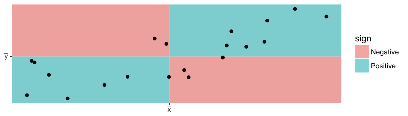
The heart of this formula is the sign of each of the \((x_i-\bar{x})(y_i-\bar{y})\) terms. If the x-value is big (greater than \(\bar{x}\)) and the y-value is large (greater than \(\bar{y}\)), then after multiplication, the result is positive. Likewise if the x-value is small and the y-value is small, both standardized values are negative and therefore after multiplication the result is positive. If a large x-value is paired with a small y-value, then the first value is positive, but the second is negative and so the multiplication result is negative.
We will define a similar quantity for two random variables.
\[Cov(X,Y) = E\left[ \big(X-E(X)\big)\big(Y-E(Y)\big) \right]\]
- Prove that for random variables \(X\) and \(Y\) such that \(Var(X)<\infty\) and \(Var(Y) < \infty\), \[Cov(X,Y) = E(XY) - E(X)E(Y)\]
\[Cov(X,X) = E(XX)-E(X)E(X) = E\left(X^2\right) - \left[ E(X) \right]^2\] In fact, we can consider \(Var(X)\) as a special case of \(Cov(X,Y)\).
- Cauchy-Schwartz Inequality. Let \(X\) and \(Y\) be random variables, each with finite variances. Show that \(\left[ E(XY) \right]^2 \le E(X^2)E(Y^2)\). Hint: Observe that \(E\left[ (tX-Y)^2 \right] \ge 0\) for any real value \(t\) and therefore \[t^2E(X^2) -2tE(XY) + E(Y) > 0\] This a polynomial of degree \(2\) in \(t\) but has no roots. Combine this fact with the quadradic equation to achieve the desired result.
Use the Cauchy-Schwartz Inequality to show that \[-1 \le \rho(X,Y) \le 1\]
Prove that if \(X\) and \(Y\) are independent random variables, each with finite variances, then \(Cov(X,Y)=0\).
Show that the preceding statement is not an “if and only if” statement by considering the following case. Let be uniformly \(X\) distributed on the integers \(-1, 0,\) and \(1\). Let \(Y=X^2\). Show that \(X\) and \(Y\) are not independent but that \(Cov(X,Y)=0\).
Prove that for random variables \(X\) and \(Y\) and constants \(a,b,c\) and \(d\) that \[Cov( aX+b, cY+d) = ac\,Cov(X,Y)\]
Prove that for random variables \(X\) and \(Y\) \[Var( X + Y) = Var(X) + Var(Y) + 2\,Cov(X,Y)\]
Prove that for random variables \(X\) and \(Y\) and constants \(a,b,\) and \(c\) that \[Var( aX + bY + c) = a^2 Var(X) + b^2 Var(Y) + 2ab\,Cov(X,Y)\]
Suppose that \(X\) and \(Y\) have a continuous joint distribution with pdf \[f(x,y) = \frac{1}{3} (x+y) \; I(0<x<1)I(0<y<2)\] Determine the value of \(Var( 2X -3Y +8 )\)
Suppose that \(X_1,X_2,\dots,X_n\) are independent and identically distributed random variables, each with \(E(X_i)=\mu\) and \(Var(X_i)=\sigma^2\). Show that the sample mean \(\bar{X} = \frac{1}{n}\sum X_i\) has expectation \(E( \bar{X} ) = \mu\) and variance \(Var(\bar{X}) = \frac{\sigma^2}{n}\).
4.7 Conditional Expectation
In many real-world scenarios, the phenomena of interest is best modeled in a “multilevel” fashion. For example, suppose that we are interested in understanding radon levels within homes and we have radon levels from thousands of houses across the US. Because houses within a county are more similar to each other than houses that are states apart, it makes sense to model the data using a multilevel approach that models each county and then the houses within the county. In this section, we will develop certain mathematical tools that will be useful for these situations.
Example Recall the Beta-Binomial hierarchical relationship where we have some observation \(X\) that is the number of successes out of \(n\) independent Bernoulli\((P)\) trials, and the probability of success \(P\) was also a random variable but with a Beta(\(\alpha\),\(\beta\)) distribution. \[X|P \sim Binomial(n,P) \;\;\;\;\;\;\textrm{where }\;\;\; P \sim Beta(\alpha, \beta)\] Recall the probability and probability density functions were \[\begin{aligned} g(x|p) &= {n \choose x} p^x (1-p)^{n-x} \;\cdot I(x\in 0,1,\dots,n)\\ f(p) &= \frac{\Gamma(\alpha,\beta)}{\Gamma(\alpha)\Gamma(\beta)} p^{\alpha-1}(1-p)^{\beta-1} \; \cdot I(0 < p < 1) \end{aligned}\]
If we regard \(P=p=0.6\) as a known quantity, then \[E(X\,|\,P=0.6) = np = n(0.60)\] However, if we don’t know the value of \(P\) and continue to consider it a random variable, then \[E(X|P) = nP\] is just a function of the random variable \(P\) and therefore \(E(X|P)\) also a random variable. We could ask questions like what is the probability density function of \(E(X|P)\) and what is the expectation of \(E(X|P)\).
Similarly we can define the conditional expectation of some function \(h(y)\) of \(Y\) as \[E( h(Y) | x ) = \int_{-\infty}^\infty h(y) \, g_2(y|x) \,dy.\]
Suppose that \(X\) and \(Y\) are continuous random variables where \(Y\) has a finite expectation. Prove that \[E\left[ E(Y|X) \right] = E(Y)\] Hint: Start with the definition of \(E(Y)\) using the double integral and joint distribution and then split the joint distribution into the product of the conditional and marginal. Finally recognize the inner integral as \(E(Y|X=x)\).
Suppose that \(X|P \sim Binomial(n,P)\) and \(P\sim Beta(\alpha=4,\beta=6)\). Find \(E(X)\). Hint: Though we haven’t proven it (yet!), the expectation of a Beta random variable is \(\alpha/(\alpha + \beta)\).
Suppose that an unknown number of individuals (denoted as \(N\)) will be independently randomly chosen for “additional screening” by the TSA. Suppose that we allow \(N\sim Poisson(\lambda)\) individuals are selected and that the probability that a selected person is female is \(0.4\). Let \(X\) denote the number of females (out of \(N\) individuals additionally screened) and so \(X|N \sim Binomial(N, p=0.4)\). Find \(E(X)\). Hint: Though we haven’t proven it yet, the variance of a Poisson random variable is also \(\lambda\).
Suppose that an unknown number of individuals (denoted as \(N\)) will be independently randomly chosen for “additional screening” by the TSA. Suppose that we allow \(N\sim Poisson(\lambda)\) individuals are selected and that the probability that a selected person is female is \(0.4\). Let \(X\) denote the number of females (out of \(N\) individuals additionally screened) and so \(X|N \sim Binomial(N, p=0.4)\). Find \(Var(X)\).
The number of defects per yard in a certain fabric, \(Y\), was known to have a Poisson distribution with parameter \(\lambda\). The parameter \(\lambda\) was assumed to be a random variable with a Exponential(1) distribution. Find \(E(Y)\) and \(Var(Y)\). Notice that \(E(\lambda)=1\) and \(1 = Var(Y|\lambda=1) < Var(Y)\).
Suppose we have random variables \(X\) and \(Y\) with joint pdf \[f(x,y) = (x+y) \, \cdot I(0 \le x \le 1)I(0 \le y \le 1)\] Find \(E(Y|X)\) and \(Var(Y|X)\). Feel free to set up all the necessary integrals and then use software to calculate them.