Chapter 7 Beyond Linearity
library(dplyr)    # data frame manipulations
library(ggplot2)  # plotting
library(caret)
library(gam)      # for loess and GAM
We will consider a simple regression problem where a flexible model is appropriate.
data('lidar', package='SemiPar')
ggplot(lidar, aes(x=range, y=logratio)) +
geom_point()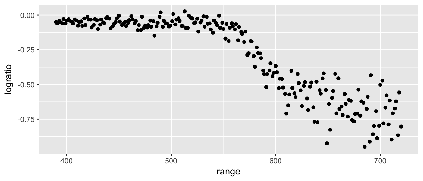 This is data from a lidar experiment (light dectection and ranging). The goal is to use the device to estimate the range at which an object is from the device operator. Light from two lasers is reflected back and the ratio of the received light from the two is observed. The exact context doesn’t matter too much, but it is a nice set of data to try to fit a curve to.
7.1 Locally Weighted Scatterplot Smoothing (LOESS)
There are a number of ways to access a LOESS smooth in R. The base R function loess() works well, but has no mechanisms for using cross validation to select the tuning parameter.
#' Span: proportion of observations to be used
#' degree: the degree of polynomial we fit at each local point.
spans <- c(1, .5, .25, .1)
P <- NULL
for( i in 1:4 ){
  model <- loess(logratio ~ range, data=lidar,
                 span = spans[i], degree=2 )
  lidar$yhat <- predict(model, newdata=lidar)

  P[[i]] <-
    ggplot(lidar, aes(x=range, y=logratio)) +
    geom_point() +
    geom_line(aes(y=yhat), color='red') +
    labs(title=paste('Span =',spans[i]))
}
Rmisc::multiplot(P[[1]], P[[2]], P[[3]], P[[4]], layout = matrix(1:4, nrow=2))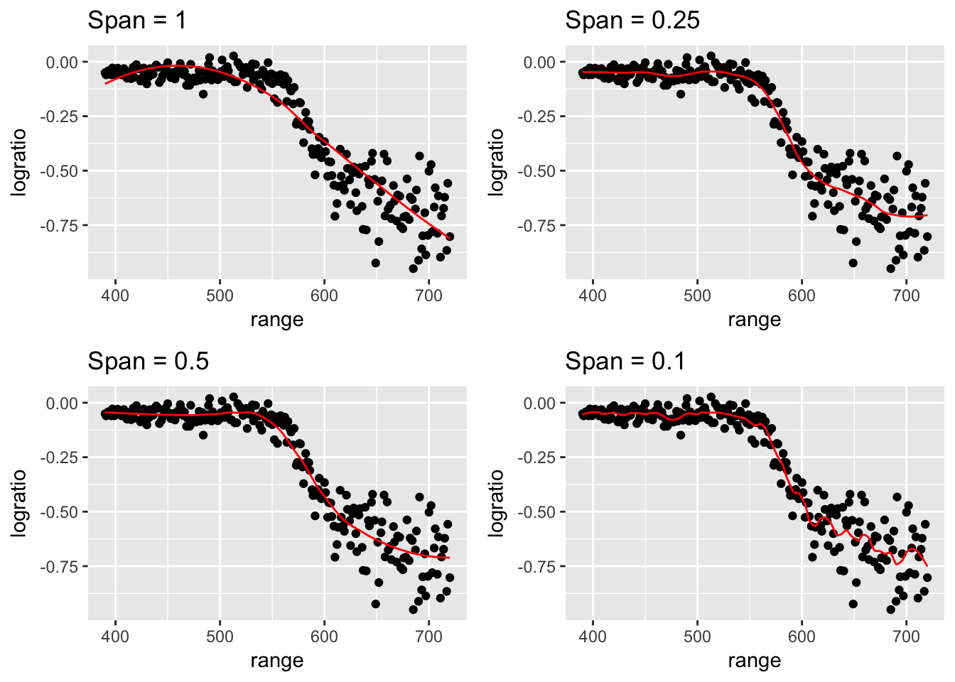
To select the tuning parameter via cross validation, we ought to jump to the caret package.
#' Span: proportion of observations to be used
#' degree: the degree of polynomial we fit at each local point.
ctrl <- trainControl( method='repeatedcv', repeats=2, number=10)
grid <- data.frame( span=seq(.01,.95,by=.02), degree=1)
model <- train(logratio ~ range, data=lidar, method='gamLoess',
               trControl=ctrl, tuneGrid=grid)

lidar$yhat <- predict(model, newdata=lidar)
ggplot(lidar, aes(x=range, y=logratio)) +
    geom_point() +
    geom_line(aes(y=yhat), color='red')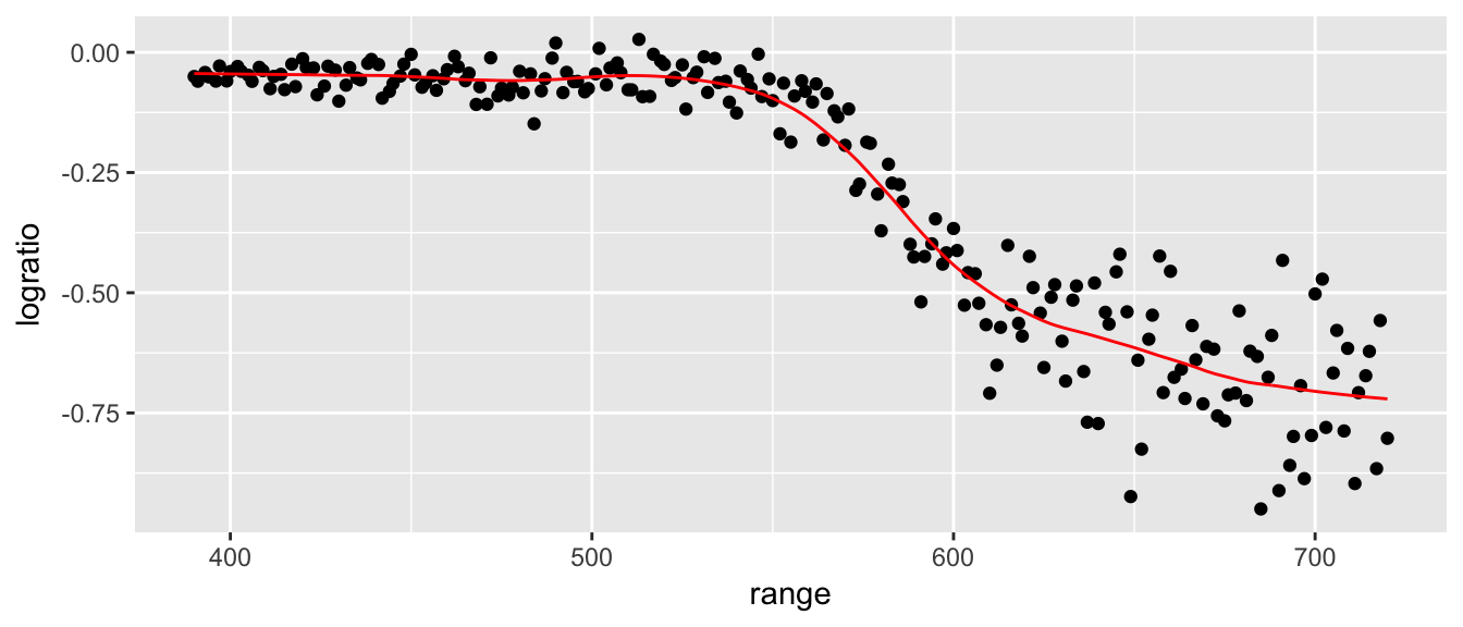
model$bestTune ## span degree
## 12 0.23 17.2 Piecewise linear
One way to allow for flexibility is to consider a segmented line where we allow the line slope to change at particular locations, which we will call breakpoints and donote them as \(\xi_1, \xi_2, \dots, \xi_K\). We will do this utilizing the truncation operator \[( u )_+ = \begin{cases} 0 \;\; \textrm{ if }\;\; u < 0 \\ u \;\; \textrm{ if } \;\; u\ge 0 \end{cases}\] and we define the truncation operator to have precedent than exponentiation so that \[(u)_+^2 = \left[ (u)_+ \right]^2\].
We can define the piecewise linear function with a single break point as \[f(x) = \beta_0 + \beta_1 x + \beta_2 (x-\xi)_+\]
Example: Suppose that we have some data we wish to fit a piecewise linear model to. The following are square root of abundance of mayflies on the Arkansas River in Colorado post clean-up for heavy metals. We are interested in how long it took for the ecosystem to reach a steady state after monitoring began.
data('Arkansas', package='SiZer')
ggplot(Arkansas, aes(x=year, y=sqrt.mayflies)) + geom_point()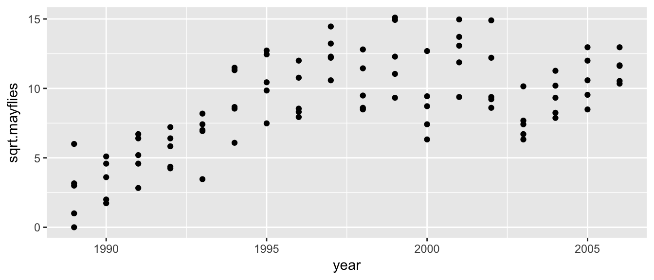
It looks like fitting a breakpoint at 1998 would be good.
n <- nrow(Arkansas)
y <- Arkansas$sqrt.mayflies
X <- cbind( rep(1,n), Arkansas$year, ifelse( Arkansas$year>=1998, (Arkansas$year-1998), 0 ) )
head(X)
## [,1] [,2] [,3]
## [1,] 1 1989 0
## [2,] 1 1989 0
## [3,] 1 1989 0
## [4,] 1 1989 0
## [5,] 1 1989 0
## [6,] 1 1990 0tail(X)## [,1] [,2] [,3]
## [85,] 1 2005 7
## [86,] 1 2006 8
## [87,] 1 2006 8
## [88,] 1 2006 8
## [89,] 1 2006 8
## [90,] 1 2006 8Next we fit the linear model, but tell the lm() command that I’ve already figured out the design matrix \(X\).
model <- lm( y ~ -1 + X )  # The -1 is because I've already included the intercept
summary(model)
##
## Call:
## lm(formula = y ~ -1 + X)
##
## Residuals:
## Min 1Q Median 3Q Max
## -4.978 -1.807 0.092 1.421 4.117
##
## Coefficients:
## Estimate Std. Error t value Pr(>|t|)
## X1 -1.939e+03 1.870e+02 -10.37 < 2e-16 ***
## X2 9.762e-01 9.378e-02 10.41 < 2e-16 ***
## X3 -1.236e+00 1.797e-01 -6.88 8.73e-10 ***
## ---
## Signif. codes: 0 '***' 0.001 '**' 0.01 '*' 0.05 '.' 0.1 ' ' 1
##
## Residual standard error: 2.211 on 87 degrees of freedom
## Multiple R-squared: 0.9477, Adjusted R-squared: 0.9459
## F-statistic: 525.7 on 3 and 87 DF, p-value: < 2.2e-16The first coefficient is the y-intercept (ie. the height at year=0), which we don’t care about. The second term is the slope prior to \(\xi=1998\), which is nearly 1. The second term is the change of slope at \(\xi=1998\) which is a decrease in slope of about \(-1.2\). So the slope of the second half of the data is slightly negative.
Arkansas$yhat <- predict(model)
ggplot(Arkansas, aes(x=year, y=sqrt.mayflies)) +
  geom_point() +
  geom_line(aes(y=yhat), color='red')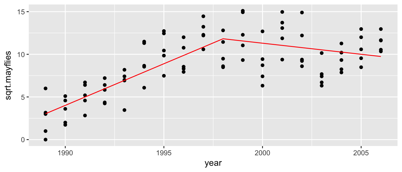
If we wanted to fit a smoother function to the data (so that there was a smooth transition at 1998), we could fit a degree 2 spline with a single breakpoint (which is generally called a knotpoint) via:
\[f(x) = \beta_0 + \beta_1 x + \beta_2 x^2 + \beta_3 (x-\xi)_+^2\]
In general we could fit a degree \(p\) spline with \(K\) knotpoints \(\xi_1,\dots,\xi_K\) as: \[f(x) = \beta_0 +\sum_{j=1}^p \beta_j x^j + \sum_{k=1}^{K} \beta_{p+k} (x-\xi_k)_+^p\]
To demonstrate, we could fit the Arkansas data with degree two spline with two knotpoints via:
X <- cbind( rep(1,n),
            Arkansas$year,
            Arkansas$year^2,
            ifelse( Arkansas$year>=1998, (Arkansas$year-1998)^2, 0 ),
            ifelse( Arkansas$year>=2003, (Arkansas$year-2003)^2, 0 ) )

model <- lm( y ~ -1 + X )  # The -1 is because I've already included the intercept

Arkansas$yhat = predict(model)
ggplot(Arkansas, aes(x=year, y=sqrt.mayflies)) +
  geom_point() +
  geom_line(aes(y=yhat), color='red')
It is a bit annoying to have to create the design matrix by hand, and the truncated polynomial basis is numerically a bit unstable, so instead we’ll use an alternate basis for splines, the B-spline basis functions. For a spline of degree \(p\) and \(K\) knotpoints \(\xi_1,\dots,\xi_K\), we replace the \(1, x, x^2, \dots, x^p, (x-\xi_1)_+^p, \dots (x-\xi_K)_+^2\) functions with other functions that are more numerically stable but equivalent. These basis functions can be generated via the bs() function
model <- lm( sqrt.mayflies ~ bs(year, degree = 2, knots = c(1998, 2003)), data=Arkansas )

Arkansas$yhat = predict(model)
ggplot(Arkansas, aes(x=year, y=sqrt.mayflies)) +
  geom_point() +
  geom_line(aes(y=yhat), color='red')
7.3 Smoothing Splines
The question of where the knot points should be located is typically addressed by putting a large number of knot points along the coefficient axis and then using a model selection routine (e.g. LASSO) to select which \(\beta_j\) terms should be pushed to zero.
The way we will control the wiggliness of the resulting function is by the estimated degrees of freedom of the smoother function, ie trace\((S)\). The higher the degrees of freedom, the more wiggly the resulting function will be.
To fit these models, we will use the gam package. Behind the scenes, gam will take the tuning parameter \(df\) and decide how best to constrain the \(\beta\) values so that the resulting smoother function has the appropriate degrees of freedom.
i <- 1
for( df in c(2,5,10,20) ){
  model <- gam( sqrt.mayflies ~ s(year, df), data=Arkansas )
  Arkansas$yhat <- predict(model)
  P[[i]] <- ggplot(Arkansas, aes(x=year)) +
    geom_point( aes(y=sqrt.mayflies) ) +
    geom_line( aes(y=yhat), color='red') +
    labs(title=paste('DF =',df))
  i <- i + 1
}
Rmisc::multiplot(P[[1]], P[[2]], P[[3]], P[[4]], cols = 2)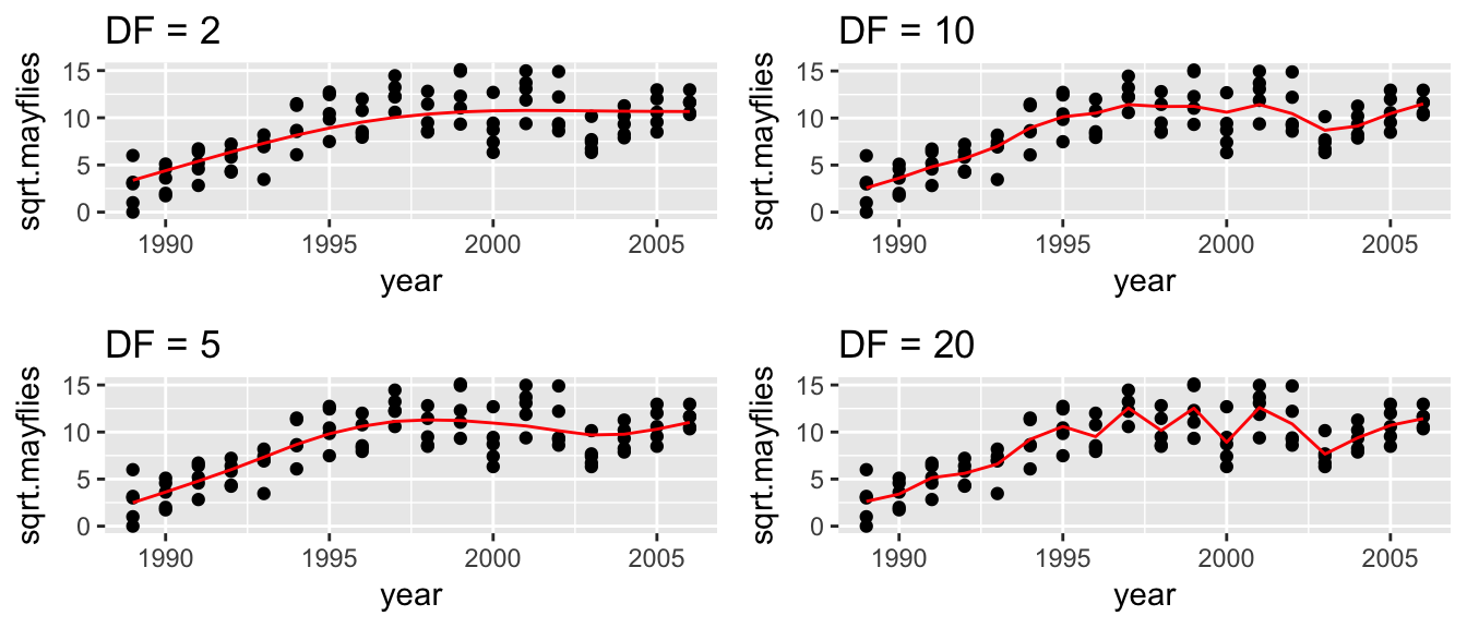
Just looking at the graphs, I think that a smoother with between 5 and 10 degrees of freedom would be best, but I don’t know which. To decide on our tuning parameter, as always we will turn to cross-validation.
ctrl <- trainControl( method='repeatedcv', repeats=10, number=4 )
grid <- data.frame(df=1:20)
model <- train( sqrt.mayflies ~ year, data=Arkansas, method='gamSpline',
                tuneGrid=grid, trControl=ctrl )

# Best tune?
model$bestTune
## df
## 14 14# OneSE best tune?
caret::oneSE(model$results,
'RMSE', # which metric are we optimizing with respect to
num=nrow(model$resample), # how many hold outs did we make
maximize=FALSE) # Is bigger == better?## [1] 3In this case, I often feel like my intuition as a scientist is at least as important as the cross-validation. I know that the ecosystem is recovering to a “steady state”, but I know that “steady state” has pretty high year-to-year variability due to severity of winter, predator/prey cycles, etc. So I want it to be flexible but not too much and I might opt for around 4 or 5.
7.4 GAMS
The smoothing splines above are quite interesting, but we would like to incorporate it into the standard modeling techniques. Considering we were able to fit a smoothing spline by simply creating the appropriate design matrix, it isn’t surprising that we could add it to the usual linear model analyses.
In the faraway package, there is a data set called ozone that has atmospheric ozone concentration and meteorology in the Los Angeles Basin in 1976. We will consider using wind speed, daily maximum temperature and Day-of-Year to model daily ozone levels.
data('ozone', package='faraway')
ozone <- ozone %>% dplyr::select(O3, wind, temp, doy)
pairs(ozone)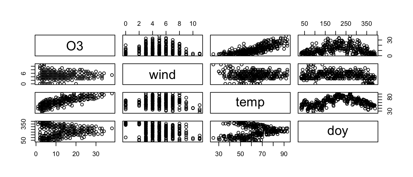
Let’s fit a smoother to temperature and day-of-year, but a standard linear relationship to wind.
library(mgcv)   # for some reason the gam library fails when I build the book.
model <- mgcv::gam(O3 ~ wind + s(temp) + s(doy), data=ozone)
mgcv::summary.gam(model)
##
## Family: gaussian
## Link function: identity
##
## Formula:
## O3 ~ wind + s(temp) + s(doy)
##
## Parametric coefficients:
## Estimate Std. Error t value Pr(>|t|)
## (Intercept) 13.8365 0.6861 20.167 < 2e-16 ***
## wind -0.4250 0.1326 -3.205 0.00149 **
## ---
## Signif. codes: 0 '***' 0.001 '**' 0.01 '*' 0.05 '.' 0.1 ' ' 1
##
## Approximate significance of smooth terms:
## edf Ref.df F p-value
## s(temp) 4.379 5.423 54.898 < 2e-16 ***
## s(doy) 5.382 6.555 7.871 2.47e-08 ***
## ---
## Signif. codes: 0 '***' 0.001 '**' 0.01 '*' 0.05 '.' 0.1 ' ' 1
##
## R-sq.(adj) = 0.705 Deviance explained = 71.4%
## GCV = 19.66 Scale est. = 18.96 n = 330mgcv::plot.gam(model, pages=1 )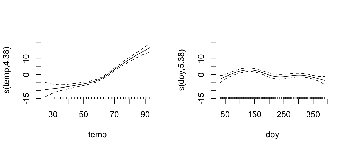
7.5 Exercises
- ISLR 7.1. It was mentioned in the chapter that a cubic regression spline with one knot at \(\xi\) can be obtained using a basis of the form \(x, x^2, x^3, (x-\xi)^3_+\), where \((x-\xi)^3_+ = (x-\xi)^3\) if \(x>\xi\) and equals \(0\) otherwise. We will now show that a function of the form \[f(x) = \beta_0 + \beta_1 x + \beta_2 x^2 + \beta_3 x^3 + \beta_4 (x-\xi)^3_+\] is indeed a cubic regression spline, regardless of the values of \(\beta_0, \beta_1, \beta_2, \beta_3,\) and \(\beta_4\). To do this we need to show that \(f(x)\) is a degree 3 polynomial on each piece and that the 0\(^{th}\), 1\(^{st}\), and 2\(^{nd}\) derivatives are continuous at \(\xi\).
- Find the cubic polynomial \[f_1(x) = a_1 + b_1 x + c_1 x^2 + d_1 x^3\] such that \(f(x) = f_1(x)\) for all \(x\le\xi\). Express \(a_1, b_1, c_1, d_1\) in terms of \(\beta_0, \beta_1, \beta_2, \beta_3, \beta_4\). Hint: this is just defining \(a_1\) as \(\beta_0\), etc.
- Find a cubic polynomial \[f_2(x) = a_2 + b_2 x + c_2 x^2 + d_2 x^3\] such that \(f(x) = f_2(x)\) for all \(x>\xi\). Express \(a_2, b_2, c_2, d_2\) in terms of \(\beta_0, \beta_1, \beta_2, \beta_3,\) and \(\beta_4\). We have now established that \(f(x)\) is a piecewise polynomial.
- Show that \(f_1(\xi) = f_2(\xi)\). That is, \(f(x)\) is continous at \(\xi\).
- Show that \(f_1'(\xi) = f_2'(\xi)\). That is, \(f'(x)\) is continous at \(\xi\).
- Show that \(f_1''(\xi) = f_2''(\xi)\). That is, \(f''(x)\) is continous at \(\xi\). Therefore, \(f(x)\) is indeed a cubic spline.
- ISLR 7.5. Consider two curves, \(\hat{g}_1\) and \(\hat{g}_2\), defined by \[\hat{g}_1 = \textrm{arg} \min_g \left( \sum_{i=1}^n \left(y_i -g(x_i)\right)^2 + \lambda \int \left[ g^{(3)}(x) \right]^2 \, dx \right),\] \[\hat{g}_2 = \textrm{arg} \min_g \left( \sum_{i=1}^n \left(y_i -g(x_i)\right)^2 + \lambda \int \left[ g^{(4)}(x) \right]^2 \, dx \right),\] where \(g^{(m)}\) represents the \(m\)th derivative of \(g\).
- As \(\lambda \to \infty\), will \(\hat{g}_1\) or \(\hat{g}_2\) have the smaller training RSS?
- As \(\lambda \to \infty\), will \(\hat{g}_1\) or \(\hat{g}_2\) have the smaller test RSS?
- For \(\lambda=0\), will \(\hat{g}_1\) or \(\hat{g}_2\) have the smaller training and test RSS?
In the package SemiPar there is a dataset called lidar which gives the following data:
data('lidar', package='SemiPar') ggplot(lidar, aes(x=range, y=logratio)) + geom_point()- Using the
lm()command andbs()command for generating a design matrix, fit a piecewise linear spline with two knot points. - Fit a smoothing spline to these data using cross-validation to select the degrees of freedom.
- Using the
ISLR 7.8. Fit some of the non-linear models investigated in this chapter to the
Autodata set. Is there evidence for non-linear relationships in this data set? Create some informative plots to justify your answer. For this data set, we are looking at the response variable ofmpgvs the other covariates, of which,displacement,horsepower,weight, andaccelerationare continuous. Let’s look and see which have a non-linear relationship withmpg.