Chapter 8 Classification and Regression Trees
library(dplyr)
library(ggplot2)
library(ISLR)
library(tree)
library(rpart)
library(rpart.plot)
8.1 Decision Trees
There are two primary packages that you could use to fit decision trees. The package tree is a relatively simple package to use, but its graphical output isn’t great. Alternatively the package rpart (which is a shortened version of Recursive Partitioning), has a great many options and has another package that is devoted to just making good graphics. My preference is to use rpart, but we will show how to use both.
8.1.1 Regression Examples
We begin our discussion of regression trees by considering an example where we attempt to predict a vehicle’s fuel efficiency (city miles) using characteristics of the vehicle.
data('mpg', package='ggplot2')
mpg <- mpg %>%
  mutate(drv=factor(drv), cyl = factor(cyl) )
str(mpg)
## Classes 'tbl_df', 'tbl' and 'data.frame': 234 obs. of 11 variables:
## $ manufacturer: chr "audi" "audi" "audi" "audi" ...
## $ model : chr "a4" "a4" "a4" "a4" ...
## $ displ : num 1.8 1.8 2 2 2.8 2.8 3.1 1.8 1.8 2 ...
## $ year : int 1999 1999 2008 2008 1999 1999 2008 1999 1999 2008 ...
## $ cyl : Factor w/ 4 levels "4","5","6","8": 1 1 1 1 3 3 3 1 1 1 ...
## $ trans : chr "auto(l5)" "manual(m5)" "manual(m6)" "auto(av)" ...
## $ drv : Factor w/ 3 levels "4","f","r": 2 2 2 2 2 2 2 1 1 1 ...
## $ cty : int 18 21 20 21 16 18 18 18 16 20 ...
## $ hwy : int 29 29 31 30 26 26 27 26 25 28 ...
## $ fl : chr "p" "p" "p" "p" ...
## $ class : chr "compact" "compact" "compact" "compact" ...t <- tree( cty ~ displ + year + cyl + drv, data=mpg)
plot(t) # show the structure
text(t, pretty = TRUE) # add text describing the split decisions.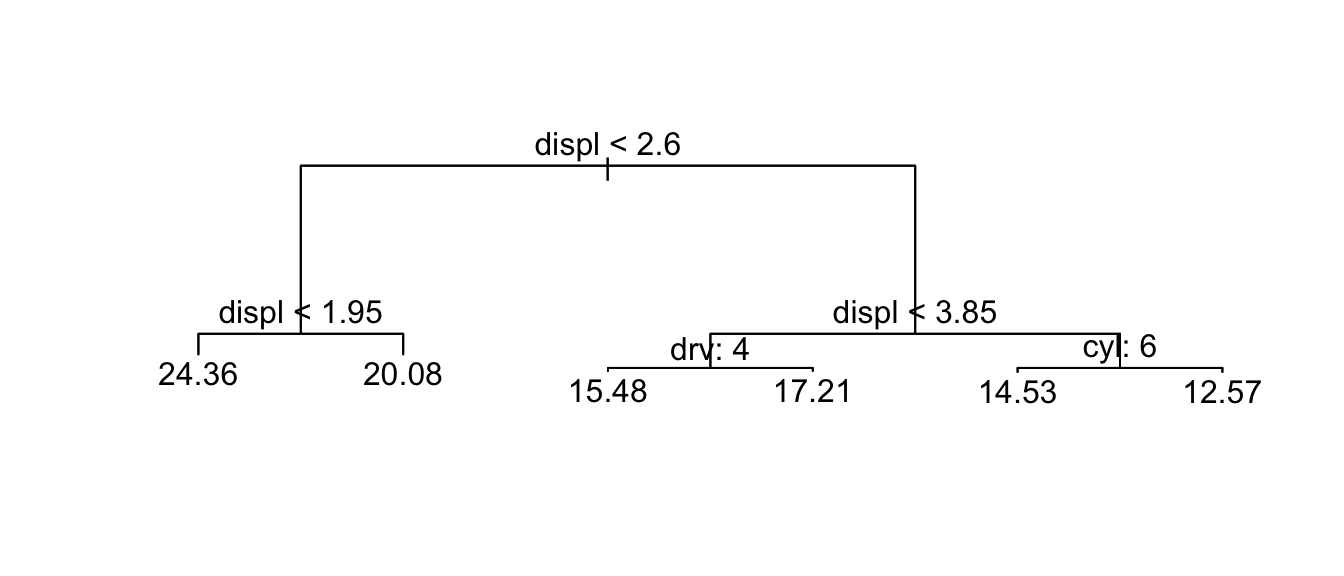
Branch lengths are proportional to the decrease in impurity of the leaf. So the longer the branch length, the more the RSS decreased for observations beneath. The splits are done so the if the evaluation of the split criterion is true, you go to the left branch, if it is false, you take the right branch.
We can control the size of the tree returned using a few options:
mincut- The minimum number of observations to include in either child node. The default is 5.minsize- The smallest allowed node size. The default is 10.mindev- The within-node deviance must be at least this times that of the root node for the node to be split. The default is 0.01.
So if we wanted a much bigger tree, we could modify these
t <- tree( cty ~ displ + year + cyl + drv, data=mpg, mindev=0.001)
plot(t) # show the structure 
Here we chose not to add the labels because the labels would over-plot each other. On way to fix that is to force the branch lengths to be equal sized.
plot(t, type='uniform')   # show the structure
text(t)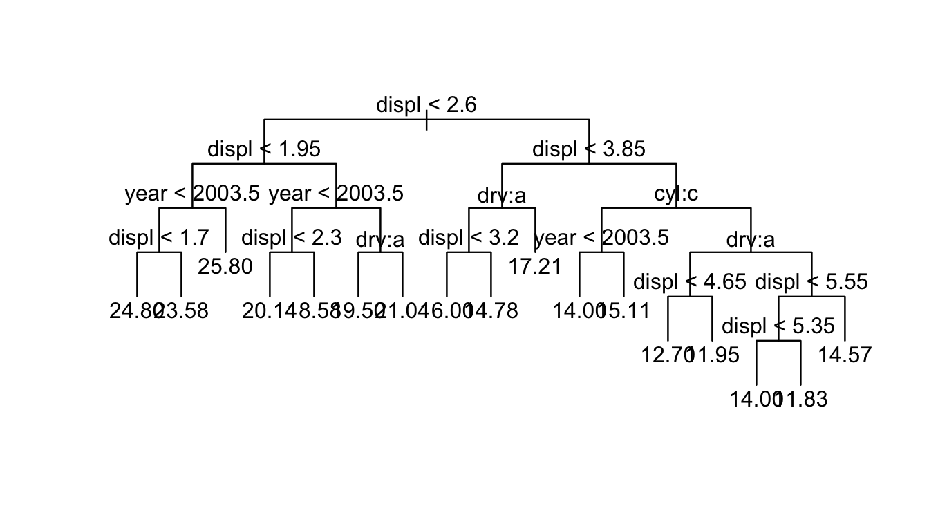
As usual, you could get predictions using the predict function and there is also a summary function
summary(t)##
## Regression tree:
## tree(formula = cty ~ displ + year + cyl + drv, data = mpg, mindev = 0.001)
## Number of terminal nodes: 17
## Residual mean deviance: 3.561 = 772.7 / 217
## Distribution of residuals:
## Min. 1st Qu. Median Mean 3rd Qu. Max.
## -7.5830 -0.9474 0.0000 0.0000 0.8571 11.4200Notice that the summary output is giving the Residual Sum of Squares as 772.7, but it is labeling it as deviance. In the regression case, the measure of model misfit is usually residual sum of squares, but in the classification setting we will using something else. Deviance is the general term we will use in both cases to denote model error, and in the regression case it is just Residual Sum of Squares.
To get the mean deviance, we are taking the deviance and dividing by \(n-p\) where \(p\) is the number of leaves.
As presented in our book, because the partition always makes the best choice at any step without looking ahead to future splits, sometimes it is advantageous to fit too large of a tree and then prune it back. To do the pruning, we consider cost complexity pruning where we consider subtrees of the full tree \(T \subset T_0\), where we create a subtree \(T\) by removing one or more nodes and merging the terminal nodes below the removed node.. We create a tuning paramter \(\alpha >0\) and seek to minimize \[\sum_{i=1}^n (y_i - \hat{y}_i)^2 + \alpha |T|\] where \(T\) is a subtree of \(T_0\), \(|T|\) is the number of terminal nodes (leaves) of the subtree, and \(\hat{y}_i\) is the predicted value for observation \(i\).
t <- tree( cty ~ displ + year + cyl + drv, data=mpg, mindev=0.001)  # Very large

# select the tree w
t.small <- prune.tree(t, best=5 )
plot(t.small); text(t.small)
Next we consider a sequence of tuning values which induces a sequence of best subtrees. The set of best subtrees can be organized by the number of terminal nodes and see the effect on the RMSE. How large a tree should we use? Cross-Validation!
cv.result <- cv.tree(t, K=10)
plot(cv.result)
t.small <- prune.tree(t, best=5)
plot(t.small)
text(t.small) 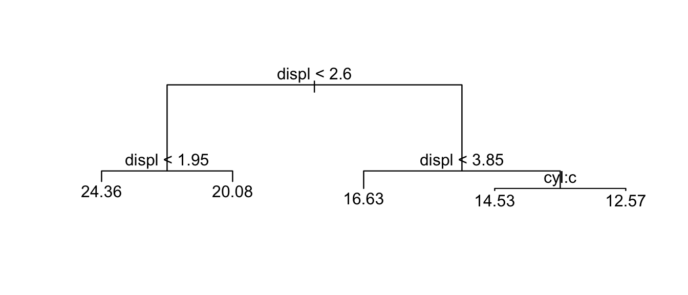
summary(t.small)##
## Regression tree:
## snip.tree(tree = t, nodes = c(14L, 4L, 5L, 15L, 6L))
## Variables actually used in tree construction:
## [1] "displ" "cyl"
## Number of terminal nodes: 5
## Residual mean deviance: 4.21 = 964.2 / 229
## Distribution of residuals:
## Min. 1st Qu. Median Mean 3rd Qu. Max.
## -8.3640 -1.4860 0.3651 0.0000 1.3650 10.6400An example where pruning behaves interestingly is where the first cut is practically useless, but allows for highly successful subsequent cuts. In the following example we have:
set.seed(289656)
n <- 10
data <- expand.grid(x1 = seq(0,1.99,length.out=n),
                    x2 = seq(0,1.99, length.out=n)) %>%
  mutate(y = abs(floor(x1) + floor(x2) -1) + rnorm(n^2, sd=.2) )

ggplot(data, aes(x=x1, y=x2, fill=y)) + geom_tile() +
    scale_fill_gradient2(low = 'blue', mid = 'white', high='red', midpoint = .5)
In this case we want to divide the region into four areas, but the first division will be useless.
t <- tree(y ~ x1 + x2, data=data)
summary(t)  # Under the usual rules, tree() wouldn't select anything
##
## Regression tree:
## tree(formula = y ~ x1 + x2, data = data)
## Variables actually used in tree construction:
## character(0)
## Number of terminal nodes: 1
## Residual mean deviance: 0.2827 = 27.98 / 99
## Distribution of residuals:
## Min. 1st Qu. Median Mean 3rd Qu. Max.
## -0.81730 -0.49640 -0.03085 0.00000 0.49770 0.89280t <- tree(y ~ x1 + x2, data=data, mindev=0.0001)
plot(t); text(t)
If we try to prune it back to a tree with 4 or fewer terminal nodes, the penalty for node size is overwhelmed by the decrease in deviance and we will stick with the larger tree.
t.small <- prune.tree(t, best=2)
plot(t.small);
text(t.small)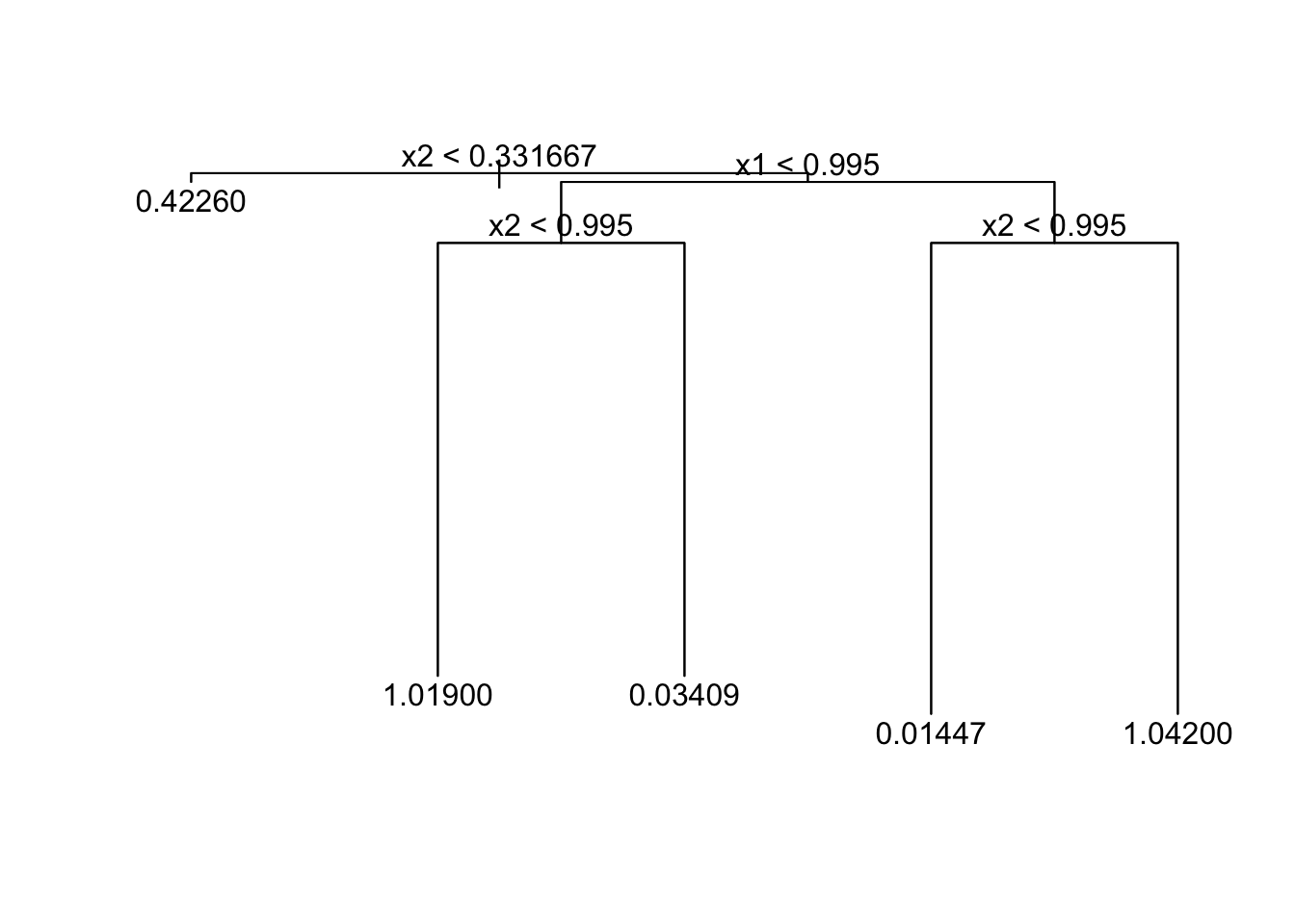
As a second example, we will consider predicting the price of a diamond based on its carat size, cut style, color and clarity quality.
data('diamonds', package='ggplot2')
t <- tree( price ~ carat+cut+color+clarity, data=diamonds)
plot(t)
text(t)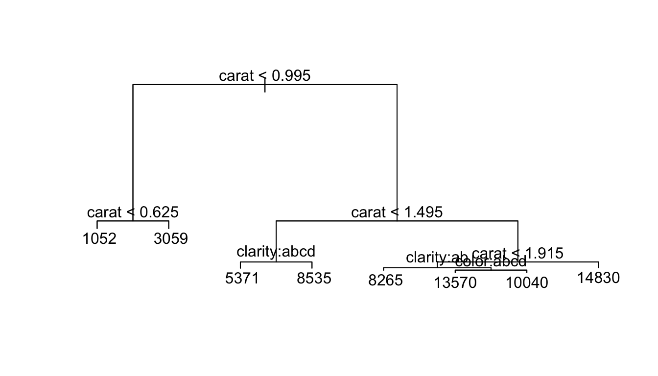
t.small <- prune.tree(t, best=5)
plot(t.small)
text(t.small, pretty = TRUE)
t.small <- prune.tree(t, best=6)
plot(t.small)
text(t.small)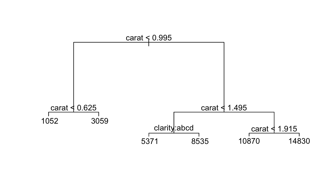
Using the package rpart and the rpart.plot packages we can fit a similar decision tree.
t2 <- rpart(cty ~ displ + year + cyl + drv, data=mpg)
rpart.plot(t2, digits=3)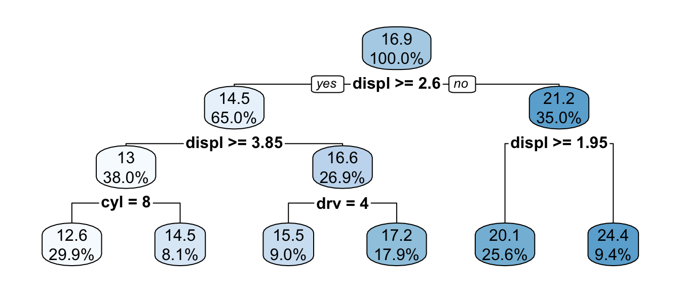
The percentages listed are the percent of data that fall into the node and its children, while the numbers represent the mean value for the terminal node or branch.
summary(t2) ## Call:
## rpart(formula = cty ~ displ + year + cyl + drv, data = mpg)
## n= 234
##
## CP nsplit rel error xerror xstd
## 1 0.57193143 0 1.0000000 1.0045185 0.12211349
## 2 0.11620091 1 0.4280686 0.4350170 0.06264448
## 3 0.06988131 2 0.3118677 0.3546300 0.06362643
## 4 0.01353184 3 0.2419864 0.2703396 0.04345028
## 5 0.01002137 4 0.2284545 0.2525780 0.04363579
## 6 0.01000000 5 0.2184331 0.2485982 0.04352400
##
## Variable importance
## displ cyl drv
## 47 38 14
##
## Node number 1: 234 observations, complexity param=0.5719314
## mean=16.85897, MSE=18.03567
## left son=2 (152 obs) right son=3 (82 obs)
## Primary splits:
## displ < 2.6 to the right, improve=0.571931400, (0 missing)
## cyl splits as RRLL, improve=0.539318200, (0 missing)
## drv splits as LRL, improve=0.444882000, (0 missing)
## year < 2003.5 to the right, improve=0.001386243, (0 missing)
## Surrogate splits:
## cyl splits as RRLL, agree=0.970, adj=0.915, (0 split)
## drv splits as LRL, agree=0.744, adj=0.268, (0 split)
##
## Node number 2: 152 observations, complexity param=0.1162009
## mean=14.5, MSE=6.25
## left son=4 (89 obs) right son=5 (63 obs)
## Primary splits:
## displ < 3.85 to the right, improve=0.516219000, (0 missing)
## cyl splits as R-RL, improve=0.508013900, (0 missing)
## drv splits as LRL, improve=0.419047600, (0 missing)
## year < 2003.5 to the right, improve=0.000997921, (0 missing)
## Surrogate splits:
## cyl splits as R-RL, agree=0.875, adj=0.698, (0 split)
## drv splits as LRL, agree=0.836, adj=0.603, (0 split)
##
## Node number 3: 82 observations, complexity param=0.06988131
## mean=21.23171, MSE=10.44631
## left son=6 (60 obs) right son=7 (22 obs)
## Primary splits:
## displ < 1.95 to the right, improve=3.442962e-01, (0 missing)
## drv splits as LR-, improve=1.274993e-01, (0 missing)
## year < 2003.5 to the left, improve=5.298225e-05, (0 missing)
##
## Node number 4: 89 observations, complexity param=0.01353184
## mean=12.98876, MSE=3.471784
## left son=8 (70 obs) right son=9 (19 obs)
## Primary splits:
## cyl splits as --RL, improve=0.18482570, (0 missing)
## displ < 4.3 to the right, improve=0.16715450, (0 missing)
## drv splits as LRR, improve=0.09757236, (0 missing)
## year < 2003.5 to the left, improve=0.01677120, (0 missing)
## Surrogate splits:
## displ < 4.1 to the right, agree=0.966, adj=0.842, (0 split)
##
## Node number 5: 63 observations, complexity param=0.01002137
## mean=16.63492, MSE=2.390527
## left son=10 (21 obs) right son=11 (42 obs)
## Primary splits:
## drv splits as LRR, improve=0.28082840, (0 missing)
## displ < 3.65 to the right, improve=0.02618858, (0 missing)
## year < 2003.5 to the left, improve=0.01832723, (0 missing)
## Surrogate splits:
## cyl splits as L-R-, agree=0.746, adj=0.238, (0 split)
## displ < 2.75 to the left, agree=0.698, adj=0.095, (0 split)
##
## Node number 6: 60 observations
## mean=20.08333, MSE=1.676389
##
## Node number 7: 22 observations
## mean=24.36364, MSE=20.95868
##
## Node number 8: 70 observations
## mean=12.57143, MSE=3.216327
##
## Node number 9: 19 observations
## mean=14.52632, MSE=1.407202
##
## Node number 10: 21 observations
## mean=15.47619, MSE=0.9160998
##
## Node number 11: 42 observations
## mean=17.21429, MSE=2.120748The default tuning parameters that control how large of a tree we fit are slightly different than in tree.
minsplitThe minimum number of observations that must exist in a node in order for a split to be attempted. The default is 20.cpThe Complexity Parameter. Any split that does not decrease the overall deviance by a factor ofcpis not attempted. The default is 0.01. This should be interpreted as the percentage of the overall dataset deviance.maxdepthSet the maximum depth of any node of the final tree, with the root node counted as depth 0. The default is 30.
t2 <- rpart(cty ~ displ + year + cyl + drv, data=mpg, cp=.001)
rpart.plot(t2, digits=3)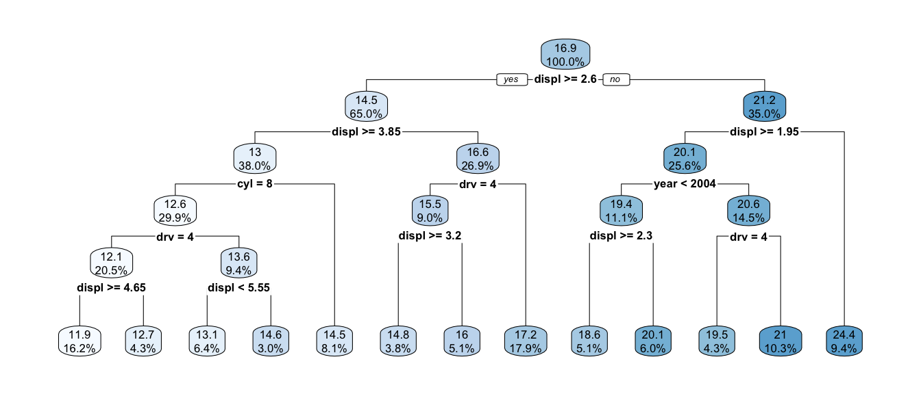
As usual we can prune the tree in the standard way using cross validation to pick the best size.
t2 <- rpart(cty ~ displ + year + cyl + drv, data=mpg, cp=.0001, xval=10) # xval = Num Folds for CV
printcp( t2 )
##
## Regression tree:
## rpart(formula = cty ~ displ + year + cyl + drv, data = mpg, cp = 1e-04,
## xval = 10)
##
## Variables actually used in tree construction:
## [1] cyl displ drv year
##
## Root node error: 4220.3/234 = 18.036
##
## n= 234
##
## CP nsplit rel error xerror xstd
## 1 0.57193143 0 1.00000 1.00889 0.122806
## 2 0.11620091 1 0.42807 0.43798 0.063138
## 3 0.06988131 2 0.31187 0.35566 0.064081
## 4 0.01353184 3 0.24199 0.28337 0.045736
## 5 0.01002137 4 0.22845 0.25864 0.045389
## 6 0.00790113 5 0.21843 0.25199 0.045609
## 7 0.00473939 6 0.21053 0.24140 0.045455
## 8 0.00397526 7 0.20579 0.23977 0.045460
## 9 0.00372368 8 0.20182 0.23346 0.045447
## 10 0.00233880 9 0.19809 0.22788 0.045518
## 11 0.00182036 10 0.19575 0.22591 0.045514
## 12 0.00106257 11 0.19393 0.22668 0.045876
## 13 0.00098102 12 0.19287 0.22850 0.045944
## 14 0.00057442 14 0.19091 0.22828 0.045974
## 15 0.00047562 15 0.19034 0.23002 0.045968
## 16 0.00037420 16 0.18986 0.23014 0.045967
## 17 0.00011358 17 0.18949 0.22906 0.045957
## 18 0.00010000 18 0.18937 0.22962 0.045951t2.small <- prune(t2, cp = .001)
rpart.plot(t2.small)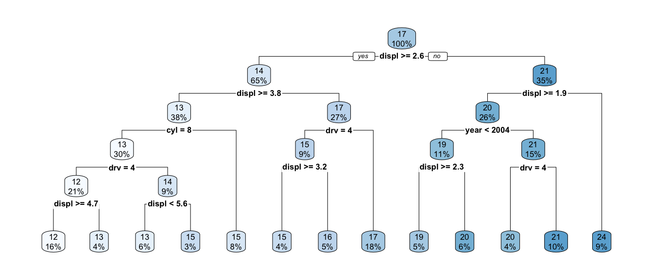
8.1.2 Classification Examples
Classification trees work identically to regression trees, only with a different measure of node purity.
data('Carseats', package='ISLR')
# make a categorical response out of Sales
Carseats <- Carseats %>%
  mutate( High = factor(ifelse(Sales >= 8, 'High','Low'))) %>%
  dplyr::select(-Sales)
Now we fit the tree using exactly the same syntax as before
set.seed(345)
my.tree <- tree( High ~ ., Carseats)
plot(my.tree)
text(my.tree)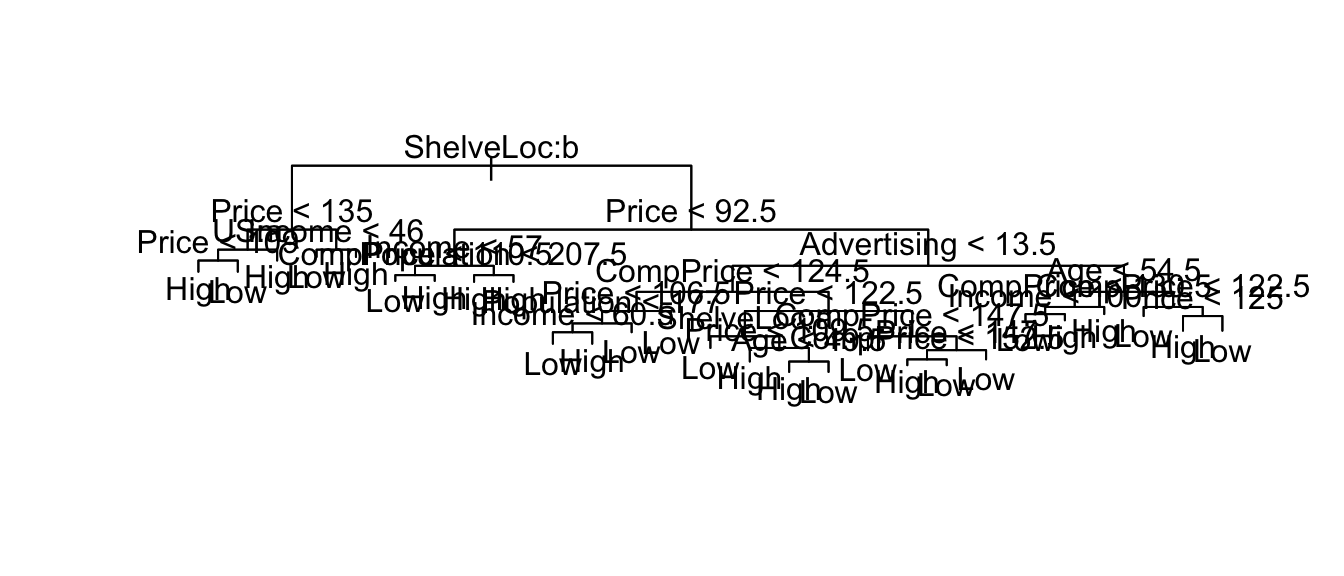
plot(my.tree, type='uniform')
text(my.tree, pretty=0)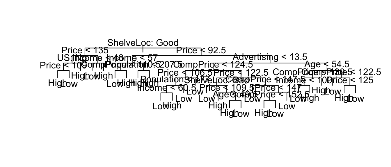
This is a very complex tree and is probably over-fitting the data. Lets use cross-validation to pick the best size tree.
# Start with the overfit tree
my.tree <- tree( High ~ ., Carseats)

# then prune using 10 fold CV where we assess on the misclassification rate
cv.tree <- cv.tree( my.tree, FUN=prune.misclass, K=10)
cv.tree
## $size
## [1] 27 26 24 22 19 17 14 12 7 6 5 3 2 1
##
## $dev
## [1] 104 105 105 101 101 97 99 91 97 99 94 98 117 165
##
## $k
## [1] -Inf 0.000000 0.500000 1.000000 1.333333 1.500000 1.666667
## [8] 2.500000 3.800000 4.000000 5.000000 7.500000 18.000000 47.000000
##
## $method
## [1] "misclass"
##
## attr(,"class")
## [1] "prune" "tree.sequence"cv.tree$size[ which.min(cv.tree$dev) ]## [1] 12# So the best tree (according to CV) has 12 leaves.# What if we prune using the deviance aka the Gini measure?
cv.tree <- cv.tree( my.tree )
cv.tree## $size
## [1] 27 26 25 24 23 22 21 20 19 17 16 14 12 11 9 8 7 6 4 3 2 1
##
## $dev
## [1] 826.9589 836.7638 836.0794 840.6605 840.2832 828.8401 828.8401
## [8] 701.3998 685.5561 665.2928 637.3993 606.2272 594.3136 563.1075
## [15] 548.7791 513.5985 500.2839 487.9836 485.8734 493.5000 497.5779
## [22] 546.9277
##
## $k
## [1] -Inf 5.487169 5.554986 5.883875 6.356830 6.770937 6.916241
## [8] 8.707541 8.849556 9.632187 9.850997 10.464072 11.246703 11.739662
## [15] 11.948400 13.135354 14.313015 18.992527 21.060122 24.699537 34.298711
## [22] 60.567546
##
## $method
## [1] "deviance"
##
## attr(,"class")
## [1] "prune" "tree.sequence"cv.tree$size[ which.min(cv.tree$dev) ]## [1] 4# The best here has 3 leaves.# Prune based on deviance
pruned.tree <- prune.tree( my.tree, best=12 )
plot(pruned.tree);
text(pruned.tree, pretty=0)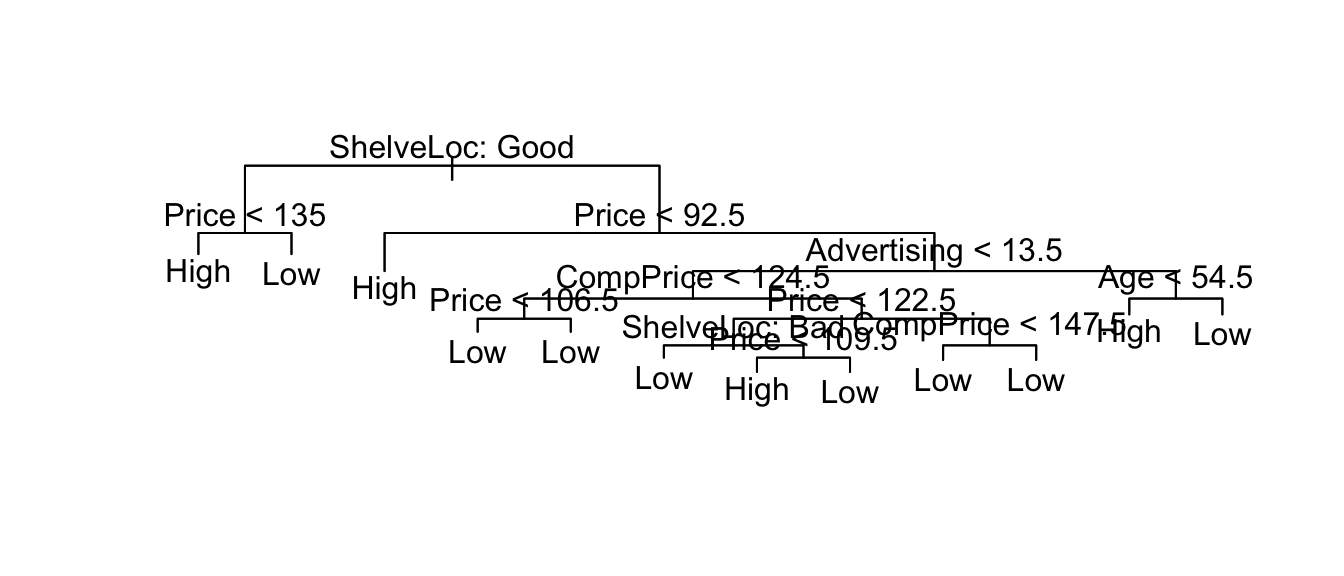
summary(pruned.tree)##
## Classification tree:
## snip.tree(tree = my.tree, nodes = c(30L, 5L, 119L, 6L, 56L, 235L,
## 4L, 31L))
## Variables actually used in tree construction:
## [1] "ShelveLoc" "Price" "Advertising" "CompPrice" "Age"
## Number of terminal nodes: 12
## Residual mean deviance: 0.7673 = 297.7 / 388
## Misclassification error rate: 0.1625 = 65 / 400# Prune based on misclassification
pruned.tree <- prune.tree( my.tree, best=12, method='misclas' )
plot(pruned.tree);
text(pruned.tree, pretty=0)
summary(pruned.tree)##
## Classification tree:
## snip.tree(tree = my.tree, nodes = c(13L, 30L, 5L, 12L, 28L, 4L,
## 59L, 31L))
## Variables actually used in tree construction:
## [1] "ShelveLoc" "Price" "Income" "Advertising" "CompPrice"
## [6] "Age"
## Number of terminal nodes: 12
## Residual mean deviance: 0.7832 = 303.9 / 388
## Misclassification error rate: 0.14 = 56 / 400# Prune based on misclassification
pruned.tree2 <- prune.tree( my.tree, best=7, method='misclas' )
plot(pruned.tree2);
text(pruned.tree, pretty=0)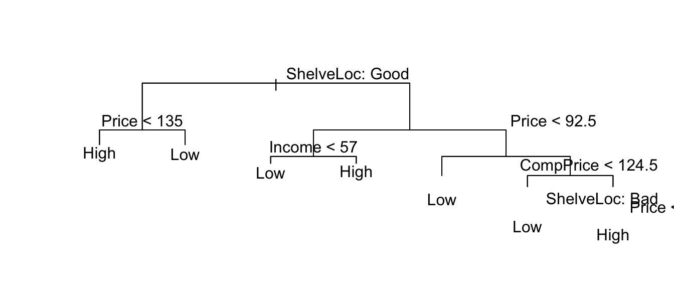
summary(pruned.tree2)##
## Classification tree:
## snip.tree(tree = my.tree, nodes = c(13L, 30L, 5L, 12L, 4L, 31L,
## 14L))
## Variables actually used in tree construction:
## [1] "ShelveLoc" "Price" "Income" "Advertising" "Age"
## Number of terminal nodes: 7
## Residual mean deviance: 0.9663 = 379.8 / 393
## Misclassification error rate: 0.1875 = 75 / 4008.2 Bagging
What is the variability tree to tree? What happens if we have different data? What if I had a different 400 observations drawn from the population?
data.star <- Carseats %>% sample_frac(replace=TRUE)
my.tree <- tree(High ~ ., data=data.star)
cv.tree <- cv.tree( my.tree, FUN=prune.misclass, K=10)
size <- cv.tree$size[ which.min(cv.tree$dev) ]
pruned.tree <- prune.tree( my.tree, best=size, method='misclas' )
plot(pruned.tree)
#text(pruned.tree, pretty=0)These are highly variable! Lets use bagging to reduce variability…
library(randomForest)
bagged <- randomForest( High ~ ., data=Carseats,
                        mtry=10,        # Number of covariates to use in each tree
                        imporance=TRUE, # Assess the importance of each covariate
                        ntree = 500)    # number of trees to grow
bagged
##
## Call:
## randomForest(formula = High ~ ., data = Carseats, mtry = 10, imporance = TRUE, ntree = 500)
## Type of random forest: classification
## Number of trees: 500
## No. of variables tried at each split: 10
##
## OOB estimate of error rate: 19%
## Confusion matrix:
## High Low class.error
## High 116 48 0.2926829
## Low 28 208 0.1186441What are the most important predictors?
importance(bagged)## MeanDecreaseGini
## CompPrice 24.3272828
## Income 18.2571468
## Advertising 21.8537267
## Population 11.3755784
## Price 51.4371819
## ShelveLoc 35.9214757
## Age 20.1961257
## Education 6.6399499
## Urban 0.7463221
## US 2.4785000varImpPlot(bagged)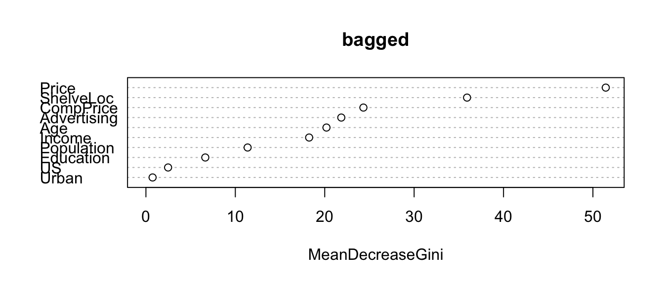
8.3 Random Forests
Where we select a different number of predictors
p <- 10
r.forest <- randomForest( High ~ ., data=Carseats,
                          mtry=p/2,        # Number of covariates to use in each tree
                          imporance=TRUE,  # Assess the importance of each covariate
                          ntree = 500)     # number of trees to grow
r.forest
##
## Call:
## randomForest(formula = High ~ ., data = Carseats, mtry = p/2, imporance = TRUE, ntree = 500)
## Type of random forest: classification
## Number of trees: 500
## No. of variables tried at each split: 5
##
## OOB estimate of error rate: 20%
## Confusion matrix:
## High Low class.error
## High 109 55 0.3353659
## Low 25 211 0.1059322Carseats$phat.High <- predict(r.forest, type='prob')[, 1]8.4 Boosting
library(gbm) # generalized boost models
boost <- gbm(High ~ .,
    data=Carseats %>% mutate(High = as.integer(High)-1),  # wants {0,1}
    distribution = 'bernoulli',  # use gaussian for regression trees
    interaction.depth = 2,  n.trees = 2000, shrinkage=.01 )
summary(boost)
##                     var    rel.inf
## phat.High     phat.High 51.5053470
## Price             Price 10.9617473
## CompPrice     CompPrice 10.4858533
## Income           Income  7.0209802
## ShelveLoc     ShelveLoc  5.4319343
## Age                 Age  4.8228414
## Advertising Advertising  3.6583231
## Population   Population  3.4534086
## Education     Education  1.8965189
## Urban             Urban  0.6234254
## US                   US  0.1396205
OK, so we have a bunch of techniques so it will pay to investigate how well they predict.
results <- NULL

for( i in 1:200){
  temp  <- Carseats
  test  <- temp %>% sample_frac(.5)
  train <- setdiff(temp, test)

  my.tree <- tree( High ~ ., data=train)
  cv.tree <- cv.tree( my.tree, FUN=prune.misclass, K=10)
  num.leaves <- cv.tree$size[which.min(cv.tree$dev)]
  pruned.tree <- prune.tree( my.tree, best=num.leaves, method='misclas' )
  yhat <- predict(pruned.tree, newdata=test, type='class')
  results <- rbind(results, data.frame(misclass=mean( yhat != test$High ),
                                       type='CV-Prune'))

  bagged <- randomForest( High ~ ., data=train, mtry=p)
  yhat   <- predict(bagged, newdata=test, type='class')
  results <- rbind(results, data.frame(misclass=mean( yhat != test$High ),
                                       type='Bagged'))

  RF     <- randomForest( High ~ ., data=train, mtry=p/2)
  yhat   <- predict(RF, newdata=test, type='class')
  results <- rbind(results, data.frame(misclass=mean( yhat != test$High ),
                                       type='RF - p/2'))

  RF     <- randomForest( High ~ ., data=train, mtry=sqrt(p))
  yhat   <- predict(RF, newdata=test, type='class')
  results <- rbind(results, data.frame(misclass=mean( yhat != test$High ),
                                       type='RF - sqrt(p)'))

  boost <- gbm(High ~ .,
    data=train %>% mutate(High = as.integer(High)-1),  # wants {0,1}
    distribution = 'bernoulli',  # use gaussian for regression trees
    interaction.depth = 2,  n.trees = 2000, shrinkage=.01 )
  yhat <- predict(boost, newdata=test, n.trees=2000, type='response')
  results <- rbind(results, data.frame(misclass=mean( round(yhat) != as.integer(test$High)-1 ),
                                       type='Boosting'))
}ggplot(results, aes(x=misclass, y=..density..)) +
geom_histogram(binwidth=0.02) +
facet_grid(type ~ .)
results %>% group_by( type ) %>%
  summarise( mean.misclass = mean(misclass),
             sd.misclass   = sd(misclass))
## # A tibble: 5 x 3
## type mean.misclass sd.misclass
## <fctr> <dbl> <dbl>
## 1 CV-Prune 0.273225 0.03420636
## 2 Bagged 0.205975 0.02880230
## 3 RF - p/2 0.199450 0.02815869
## 4 RF - sqrt(p) 0.197125 0.02690219
## 5 Boosting 0.157025 0.022651498.5 Exercises
ISLR #8.1 Draw an example (of your own invention) of a partition of a two dimensional feature space that could result from recursive binary splitting. Your example should contain at least six regions. Draw a decision tree corresponding to this partition. Be sure to label all aspects of your figures, including the regions \(R_1, R_2, \dots\), the cut-points \(t_1, t_2, \dots\), and so forth.
ISLR #8.3. Consider the Gini index, classification error, and cross-entropy in a simple classification setting with two classes. Create a single plot that displays each of these quantities as a function of \(\hat{p}_{m1}\). The \(x\)-axis should display \(\hat{p}_{m1}\), ranging from \(0\) to \(1\), and the \(y\)-axis should display the value of the Gini index, classification error, and entropy.
- ISLR #8.4 This question relates to the plots in Figure 8.12.
- Sketch the tree corresponding to the partition of the predictor space illustrated in the left-hand panel of Figure 8.12. The numbers inside the boxes indicate the mean of \(Y\) within each region.
- Create a diagram similar to the left-hand panel of Figure 8.12, using the tree illustrated in the right-hand panel of the same figure. You should divide up the predictor space into the correct regions, and indicate the mean for each region.
- ISLR #8.8 In the lab, a classification tree was applied to the
Carseatsdata set after convertingSalesinto a qualitative response variable. Now we will seek to predictSalesusing regression trees and related approaches, treating the response as a quantitative variable.Split the data set into a training set and a test set.
set.seed(9736) train <- Carseats %>% sample_frac(0.5) test <- setdiff(Carseats, train)- Fit a regression tree to the training set. Plot the tree, and interpret the results. What test error rate do you obtain?
- Use cross-validation in order to determine the optimal level of tree complexity. Does pruning the tree improve the test error rate?
- Use the bagging approach in order to analyze this data. What test error rate do you obtain? Use the
importance()function to determine which variables are most important. - Use random forests to analyze this data. What test error rate do you obtain? Use the
importance()function to determine which variables are most important. Describe the effect of \(m\), the number of variables considered at each split, on the error rate obtained. Use boosting to analyze this data. What test error rate do you obtain? Describe the effect of \(d\), the number of splits per step. Also describe the effect of changing \(\lambda\) from 0.001, 0.01, and 0.1.